# Load packages
library(googlesheets4) ## for reading data directly from Google Sheets
library(dplyr) ## for data manipulation
library(survival) ## for Kaplan-Meier estimator
library(survminer) ## for pretty survival curves
library(ggplot2) ## for other data visualization
library(stringr) ## for cleaning string fields (tropes)

# Read the data
rom_dat = read_sheet("https://docs.google.com/spreadsheets/d/10HZevTEd4CWjqIcVMbED2nkpmnXDV6NVxCKenCsUqv0/edit?usp=sharing") |>
mutate(Main_Trope = toupper(Main_Trope)) ## clean up text (make tropes all upper case)Context, Please!
Romance novels (in)famously guarantee happily ever afters (HEAs) and follow one of a few pathways (tropes) to get there. (See a nice overview of common tropes from Shondaland here.) On our first episode, we discussed Sarah’s recent side project using data to investigate whether different tropes speed up or slow down the couple getting together, even if all books are going to end with that HEA.
Behind the Scenes
Sarah collected a sample of romance novels from the last 10 years that became popular in the U.S., recording the following key variables:
Main_Trope: the primary trope employed in the novel,Page: the page on which the couple’s first kiss,Total: the total number of pages in the novel (used to normalize across books of different lengths), andPercent: the percent of the way through the book when the couple first kisses (calculated asPage/Total).
These data are publicly available! You can read them in and run the code below to replicate her analyses.
There are a lot of different tropes, and this sample captured 13 unique ones. However, a few of them were fairly uncommon, so the tropes were regrouped with others that were thematically similar (with the help of ChatGPT).
# Counts of books per original tropes
table(rom_dat$Main_Trope)
             BROTHER'S BEST FRIEND                  CELEBRITY ROMANCE
                                 4                                  2
                       FAKE DATING                   FORCED PROXIMITY
                                 4                                  2
                 FRIENDS-TO-LOVERS                    GRUMPY/SUNSHINE
                                 5                                  9
                        INSTA-LOVE                    LOVE AFTER LOSS
                                 1                                  2
               NO STRINGS ATTACHED RIVALS-TO-LOVERS/ENEMIES-TO-LOVERS
                                 1                                  8
             SECOND CHANCE ROMANCE                         SINGLE DAD
                                 8                                  1
                SURPRISE PREGNANCY
                                 1
# Create trope groupings (collapse less-frequent tropes)
rom_dat = rom_dat |>
mutate(
Main_Trope_Grouped = case_when(
Main_Trope %in% c("FAKE DATING", "FORCED PROXIMITY", "SURPRISE PREGNANCY", "NO STRINGS ATTACHED") ~ "CONTRIVED/SITUATIONAL SETUP",
Main_Trope %in% c("BROTHER'S BEST FRIEND", "CELEBRITY ROMANCE", "SINGLE DAD") ~ "POWER/STATUS/TABOO",
.default = Main_Trope
),
Kissed = 1 ## Have to define an event indicator to fit Kaplan-Meier, but all are events
) |>
filter(!(Main_Trope_Grouped %in% c("LOVE AFTER LOSS", "INSTA-LOVE"))) ## Exclude two uncommon tropes that couldn't naturally be grouped (loses 3 books)
# Counts of books per grouped tropes
table(rom_dat$Main_Trope_Grouped)
       CONTRIVED/SITUATIONAL SETUP                  FRIENDS-TO-LOVERS
                                 8                                  5
                   GRUMPY/SUNSHINE                 POWER/STATUS/TABOO
                                 9                                  7
RIVALS-TO-LOVERS/ENEMIES-TO-LOVERS              SECOND CHANCE ROMANCE
                                 8                                  8
After re-grouping, there were 6 unique values instead, with at least 5 books each.
Primary Analysis: Proportion of the Way Through the Book
Kaplan-Meier curves can be used to compare how quickly book couples first kiss (a measure of their romantic pacing). The original analysis used Percent as the measure of “how quickly” the event occurred, so that we could compare pacing across shorter/longer books by standardizing them to be on the same relative scale.
Overall (All Tropes Together)
# Fit Kaplan-Meier
fit_overall = survfit(formula = Surv(time = Percent, event = Kissed) ~ 1,
                      data = rom_dat)

# Plot overall Kaplan-Meier curve
rom_cols <- c("#E63946", "#F1A7A7", "#A26769", "#6D2E46", "#CDB4DB",  "#D96C75") ### Define pretty color palette
plot_overall = ggsurvplot(
  fit = fit_overall,
  ### Customize the look of the plot
  palette = rom_cols,
  ggtheme = theme(
    panel.background = element_rect(fill = "#F5E6E8", color = NA),
    plot.background  = element_rect(fill = "#F5E6E8", color = NA),
    panel.grid = element_line(color = "#E3D3D6"),
    axis.text = element_text(size = 20, color = "#2B1E21"),
    axis.title = element_text(size = 20, face = "bold", color = "#2B1E21")),
  xlab = "Proportion of Book Completed",
  ylab = "Probability First Kiss Has Not Occurred",
  surv.scale = "percent",
  size = 1.5,
  legend = "none",
  xlim = c(0, 1))
plot_overall$plot = plot_overall$plot +
  scale_x_continuous(labels = scales::percent) ### make x-axis a %
plot_overall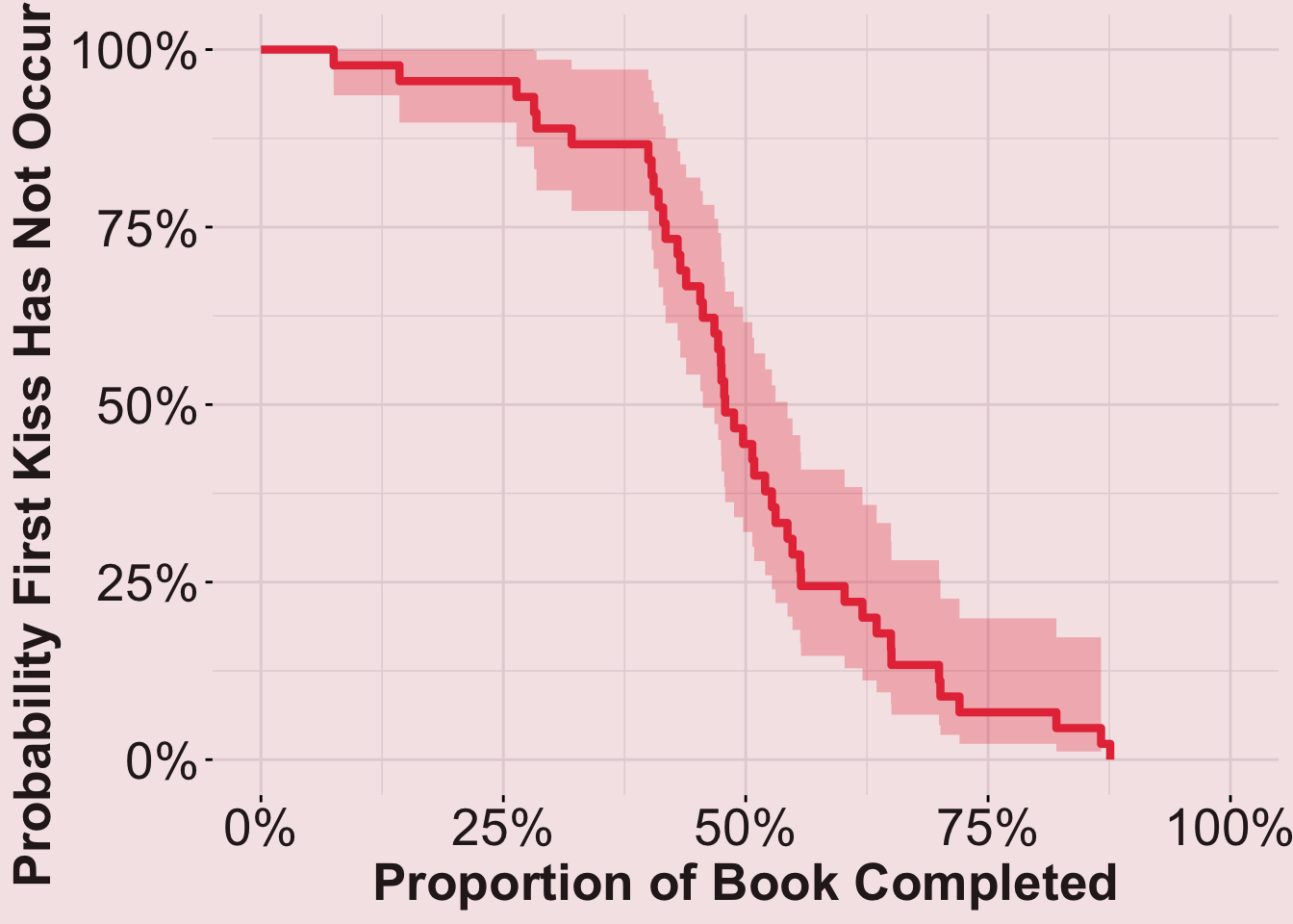
## View median survival
summary(fit_overall)$table["median"]
median
0.4787472 Results: On average, a book couple first kisses 48% of the way through the book (across all tropes), but broken down…
Stratified (Each Trope Separately)
# Fit Kaplan-Meier
fit_stratified = survfit(formula = Surv(time = Percent, event = Kissed) ~ Main_Trope_Grouped,
                         data = rom_dat)
## Plot stratified Kaplan-Meier curves
plot_stratified = ggsurvplot(
  fit = fit_stratified,
  ### Customize the look of the plot
  palette = rom_cols,
  ggtheme = theme(
    panel.background = element_rect(fill = "#F5E6E8", color = NA),
    plot.background  = element_rect(fill = "#F5E6E8", color = NA),
    panel.grid = element_line(color = "#E3D3D6"),
    axis.text = element_text(size = 20, color = "#2B1E21"),
    axis.title = element_text(size = 20, face = "bold", color = "#2B1E21")),
  xlab = "Proportion of Book Completed",
  ylab = "Probability First Kiss Has Not Occurred",
  surv.scale = "percent",
  size = 1.5,
  legend = "none",
  xlim = c(0, 1))
plot_stratified$plot = plot_stratified$plot +
  scale_x_continuous(labels = scales::percent)  ### make x-axis a %
plot_stratified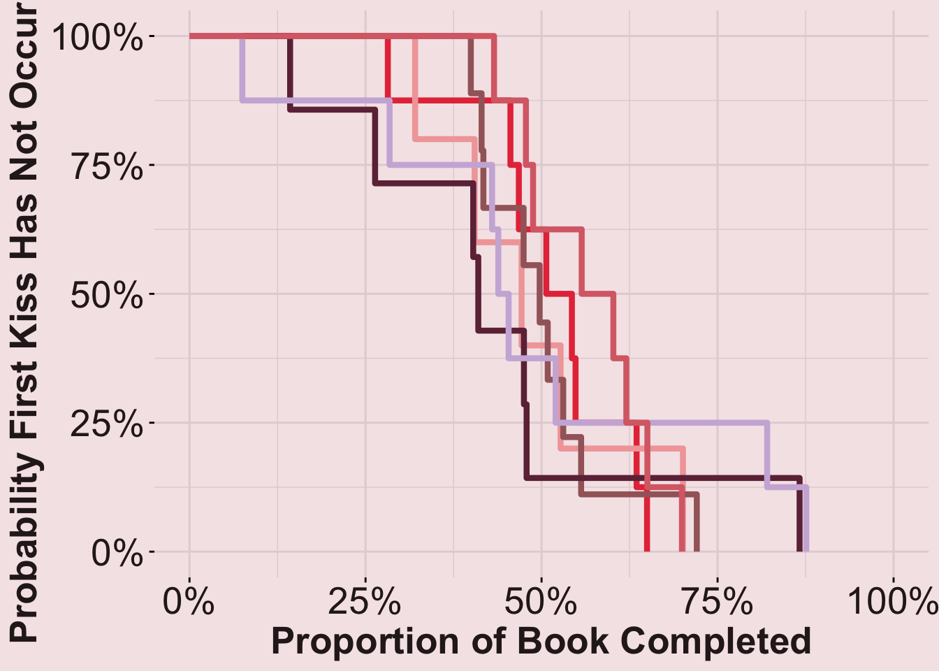
## View median survival
summary(fit_stratified)$table[, "median"]
Main_Trope_Grouped=CONTRIVED/SITUATIONAL SETUP
0.5249301
Main_Trope_Grouped=FRIENDS-TO-LOVERS
0.4716157
Main_Trope_Grouped=GRUMPY/SUNSHINE
0.4972973
Main_Trope_Grouped=POWER/STATUS/TABOO
0.4101382
Main_Trope_Grouped=RIVALS-TO-LOVERS/ENEMIES-TO-LOVERS
0.4458747
Main_Trope_Grouped=SECOND CHANCE ROMANCE
0.5794885 Results (continued): While all couples kiss by the end of the book (HEAs) and most authors seem to wait until around halfway through, some tropes seem to move faster than others.
- Fastest: First kisses happen the earliest, on average, in books belonging to the power/ status/taboo tropes (median survival = 41% through the book).
- Slowest: First kisses happen the latest, on average, in books belonging to the second chance romance trope (median survival = 58% through the book).
Secondary Analysis: Pages into the Book
While playing Reviewer 2, Lucy asked what this analysis might look like on an absolute time scale, rather than a relative one! So as a secondary analysis, Sarah repeated the overall and stratified Kaplan-Meier curves using Pages as the measure of how far into the book the first class occurred, rather than Percent.
Overall (All Tropes Together)
# Fit Kaplan-Meier curves
fit_overall2 = survfit(formula = Surv(time = Page, event = Kissed) ~ 1,
                       data = rom_dat)
## Plot overall Kaplan-Meier curve
plot_overall2 = ggsurvplot(
  fit = fit_overall2,
  ### Customize the look of the plot
  palette = rom_cols,
  ggtheme = theme(
    panel.background = element_rect(fill = "#F5E6E8", color = NA),
    plot.background  = element_rect(fill = "#F5E6E8", color = NA),
    panel.grid = element_line(color = "#E3D3D6"),
    axis.text = element_text(size = 20, color = "#2B1E21"),
    axis.title = element_text(size = 20, face = "bold", color = "#2B1E21")),
  xlab = "Pages of Book Completed",
  ylab = "Probability First Kiss Has Not Occurred",
  surv.scale = "percent",
  size = 1.5,
  legend = "none",
  xlim = c(0, max(rom_dat$Page)))
plot_overall2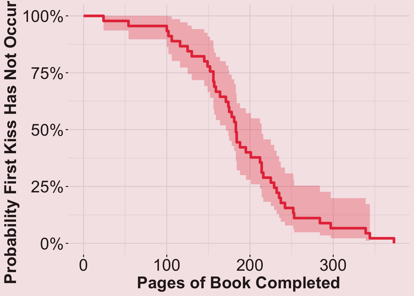
#### View median survival
summary(fit_overall2)$table["median"]
median
183 Results (continued): On average, a book couple first kisses 183% pages into the book (across all tropes), but broken down…
Stratified (Each Trope Separately)
### Stratified / using each trope separately
fit_stratified2 = survfit(formula = Surv(time = Page, event = Kissed) ~ Main_Trope_Grouped,
                          data = rom_dat)
#### Plot stratified Kaplan-Meier curves
plot_stratified2 = ggsurvplot(
  fit = fit_stratified2,
  ##### Customize the look of the plot
  palette = rom_cols,
  ggtheme = theme(
    panel.background = element_rect(fill = "#F5E6E8", color = NA),  # light pink
    plot.background  = element_rect(fill = "#F5E6E8", color = NA),
    panel.grid = element_line(color = "#E3D3D6"),
    axis.text = element_text(size = 20, color = "#2B1E21"),
    axis.title = element_text(size = 20, face = "bold", color = "#2B1E21")),
  xlab = "Proportion of Book Completed",
  ylab = "Probability First Kiss Has Not Occurred",
  surv.scale = "percent",
  size = 1.5,
  legend = "none",
  xlim = c(0, max(rom_dat$Page)))
plot_stratified2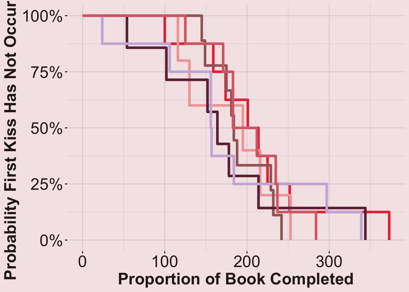
#### View median survival
summary(fit_stratified2)$table[, "median"]
Main_Trope_Grouped=CONTRIVED/SITUATIONAL SETUP
207.5
Main_Trope_Grouped=FRIENDS-TO-LOVERS
195.0
Main_Trope_Grouped=GRUMPY/SUNSHINE
184.0
Main_Trope_Grouped=POWER/STATUS/TABOO
164.0
Main_Trope_Grouped=RIVALS-TO-LOVERS/ENEMIES-TO-LOVERS
156.5
Main_Trope_Grouped=SECOND CHANCE ROMANCE
197.5 Results (continued): Interestingly, the tropes were ordered differently by the average length, in pages, to the first kiss than they were when ordered by the percent of the way into the book.
- Fastest: First kisses happen the earliest, on average, in books belonging to the rivals- or enemies-to-lovers (median survival = 156 pages into the book).
- Slowest: First kisses happen the latest, on average, in books belonging to the contrived/situational setup trope (median survival = 208% pages into the book).
Response to Reviewer
While Lucy argued that, for readers, the absolute page scale might be more representative of their experience (e.g., how long it takes them to read 150 pages), Sarah was worried that this would be misleading if some tropes simply belong to longer books, on average.
rom_dat |>
  ggplot(aes(x = Main_Trope_Grouped, y = Total, fill = Main_Trope_Grouped)) +
  geom_bar(stat = "mean") +
  theme(
    panel.background = element_rect(fill = "#F5E6E8", color = NA),  # light pink
    plot.background  = element_rect(fill = "#F5E6E8", color = NA),
    panel.grid = element_line(color = "#E3D3D6"),
    axis.text = element_text(size = 14, color = "#2B1E21"),
    axis.title = element_text(size = 14, face = "bold", color = "#2B1E21")
    ) +
  labs(x = "Main Trope (Grouped)",
       y = "Average Number of Pages Number Per Books") +
  scale_fill_manual(values = rom_cols, guide = "none") +
  scale_x_discrete(labels = function(x) str_wrap(x, width = 10, whitespace_only = FALSE)) +
  coord_flip()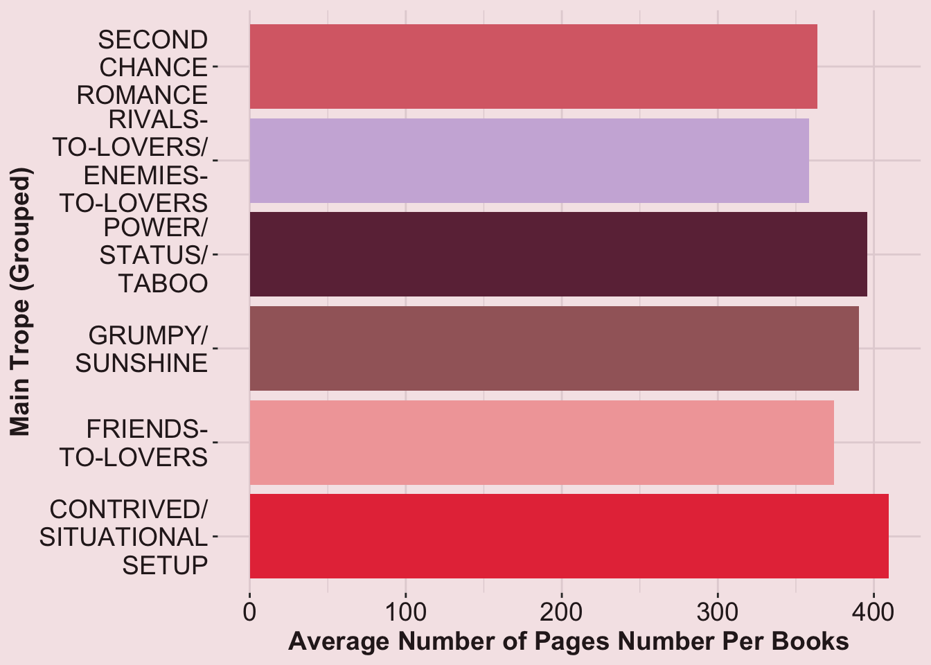
Results (continued): It looks like romance books of all sampled tropes are at least 350 pages long, on average. While those in the contrived/situational setup trope averaged over 400 pages, there were not huge differences.